BioStructures documentation
The BioStructures.jl package provides functionality to manipulate macromolecular structures, and in particular to read and write Protein Data Bank (PDB) and mmCIF files. It is designed to be used for standard structural analysis tasks, as well as acting as a platform on which others can build to create more specific tools.
It compares favourably in terms of performance to other PDB parsers - see some benchmarks. The PDB and mmCIF parsers currently read in the whole PDB without explicit errors (with one exception). Help can be found on individual functions using ?function_name.
Basics
To download a PDB file:
using BioStructures

# Stored in the current working directory by default
downloadpdb("1EN2")
To parse a PDB file into a Structure-Model-Chain-Residue-Atom framework:
julia> struc = read("/path/to/pdb/file.pdb", PDB)
ProteinStructure 1EN2.pdb with 1 models, 1 chains (A), 85 residues, 754 atoms
mmCIF files can be read into the same data structure with read("/path/to/cif/file.cif", MMCIF). If you want to read an mmCIF file into a dictionary to query yourself (e.g. to access metadata fields), use MMCIFDict:
julia> mmcif_dict = MMCIFDict("/path/to/cif/file.cif")
mmCIF dictionary with 716 fields

julia> mmcif_dict["_entity_src_nat.common_name"]
1-element Array{String,1}:
 "great nettle"
A MMCIFDict can be accessed in similar ways to a standard dictionary, and if necessary the underlying dictionary of MMCIFDict d can be accessed with d.dict. Note that the elements of the dictionary are always an Array{String,1}, even if only one value was read in or the data is numerical.
Refer to Downloading PDB files and Reading PDB files sections for more options.
The elements of struc can be accessed as follows:
| Command | Returns | Return type |
|---|---|---|
struc[1] | Model 1 | Model |
struc[1]["A"] | Model 1, chain A | Chain |
struc[1]['A'] | Shortcut to above if the chain ID is a single character | Chain |
struc["A"] | The lowest model (model 1), chain A | Chain |
struc["A"]["50"] | Model 1, chain A, residue 50 | AbstractResidue |
struc["A"][50] | Shortcut to above if it is not a hetero residue and the insertion code is blank | AbstractResidue |
struc["A"]["H_90"] | Model 1, chain A, hetero residue 90 | AbstractResidue |
struc["A"][50]["CA"] | Model 1, chain A, residue 50, atom name CA | AbstractAtom |
struc["A"][15]["CG"]['A'] | For disordered atoms, access a specific location | Atom |
Disordered atoms are stored in a DisorderedAtom container but calls fall back to the default atom, so disorder can be ignored if you are not interested in it. Disordered residues (i.e. point mutations with different residue names) are stored in a DisorderedResidue container.
The idea is that disorder will only bother you if you want it to. See the Biopython discussion for more.
Properties can be retrieved as follows:
| Function | Returns | Return type |
|---|---|---|
serial | Serial number of an atom | Int |
atomname | Name of an atom | String |
altlocid | Alternative location ID of an atom | Char |
altlocids | All alternative location IDs in a DisorderedAtom | Array{Char,1} |
x | x coordinate of an atom | Float64 |
y | y coordinate of an atom | Float64 |
z | z coordinate of an atom | Float64 |
coords | coordinates of an atom | Array{Float64,1} |
occupancy | Occupancy of an atom (default is 1.0) | Float64 |
tempfactor | Temperature factor of an atom (default is 0.0) | Float64 |
element | Element of an atom (default is " ") | String |
charge | Charge of an atom (default is " ") | String |
residue | Residue an atom belongs to | Residue |
ishetero | true if the residue or atom is a hetero residue/atom | Bool |
isdisorderedatom | true if the atom is disordered | Bool |
pdbline | PDB ATOM/HETATM record for an atom | String |
resname | Residue name of a residue or atom | String |
resnames | All residue names in a DisorderedResidue | Array{String,1} |
resnumber | Residue number of a residue or atom | Int |
sequentialresidues | Determine if the second residue follows the first in sequence | Bool |
inscode | Insertion code of a residue or atom | Char |
resid | Residue ID of an atom or residue (full=true includes chain) | String |
atomnames | Atom names of the atoms in a residue, sorted by serial | Array{String,1} |
atoms | Dictionary of atoms in a residue | Dict{String, AbstractAtom} |
isdisorderedres | true if the residue has multiple residue names | Bool |
disorderedres | Access a particular residue name in a DisorderedResidue | Residue |
chain | Chain a residue or atom belongs to | Chain |
chainid | Chain ID of a chain, residue or atom | String |
resids | Sorted residue IDs in a chain | Array{String,1} |
residues | Dictionary of residues in a chain | Dict{String, AbstractResidue} |
model | Model a chain, residue or atom belongs to | Model |
modelnumber | Model number of a model, chain, residue or atom | Int |
chainids | Sorted chain IDs in a model or structure | Array{String,1} |
chains | Dictionary of chains in a model or structure | Dict{String, Chain} |
structure | Structure a model, chain, residue or atom belongs to | ProteinStructure |
structurename | Name of the structure an element belongs to | String |
modelnumbers | Sorted model numbers in a structure | Array{Int,1} |
models | Dictionary of models in a structure | Dict{Int, Model} |
The strip keyword argument determines whether surrounding whitespace is stripped for atomname, element, charge, resname and atomnames (default true).
The coordinates of an atom can be set using x!, y!, z! and coords!.
Manipulating structures
Elements can be looped over to reveal the sub-elements in the correct order:
for mod in struc
    for ch in mod
        for res in ch
            for at in res
                # Do something
            end
        end
    end
end
Models are ordered numerically; chains are ordered by chain ID character ordering, except the empty chain is last; residues are ordered by residue number and insertion code with hetero residues after standard residues; atoms are ordered by atom serial. If you want the first sub-element you can use first. For example first(struc[1]) gets the first chain in model 1. Since the ordering of elements is defined you can use the sort function. For example sort(res) sorts a list of residues as described above, or sort(res, by=resname) will sort them alphabetically by residue name.
collect can be used to get arrays of sub-elements. collectatoms, collectresidues, collectchains and collectmodels return arrays of a particular type from a structural element or element array.
Selectors are functions passed as additional arguments to these functions. Only elements that return true when passed to all the selector are retained. For example:
| Command | Action | Return type |
|---|---|---|
collect(struc['A'][50]) | Collect the sub-elements of an element, e.g. atoms from a residue | Array{AbstractAtom,1} |
collectresidues(struc) | Collect the residues of an element | Array{AbstractResidue,1} |
collectatoms(struc) | Collect the atoms of an element | Array{AbstractAtom,1} |
collectatoms(struc, calphaselector) | Collect the C-alpha atoms of an element | Array{AbstractAtom,1} |
collectatoms(struc, calphaselector, disorderselector) | Collect the disordered C-alpha atoms of an element | Array{AbstractAtom,1} |
The selectors available are:
| Function | Acts on | Selects for |
|---|---|---|
| standardselector | AbstractAtom or AbstractResidue | Atoms/residues arising from standard (ATOM) records |
| heteroselector | AbstractAtom or AbstractResidue | Atoms/residues arising from hetero (HETATM) records |
| atomnameselector | AbstractAtom | Atoms with atom name in a given list |
| calphaselector | AbstractAtom | C-alpha atoms |
| cbetaselector | AbstractAtom | C-beta atoms, or C-alpha atoms for glycine residues |
| backboneselector | AbstractAtom | Atoms in the protein backbone (CA, N and C) |
| heavyatomselector | AbstractAtom | Non-hydrogen atoms |
| hydrogenselector | AbstractAtom | Hydrogen atoms |
| resnameselector | AbstractAtom or AbstractResidue | Atoms/residues with residue name in a given list |
| waterselector | AbstractAtom or AbstractResidue | Atoms/residues with residue name HOH |
| notwaterselector | AbstractAtom or AbstractResidue | Atoms/residues with residue name not HOH |
| disorderselector | AbstractAtom or AbstractResidue | Atoms/residues with alternative locations |
To create a new atomnameselector or resnameselector:
cdeltaselector(at::AbstractAtom) = atomnameselector(at, ["CD"])It is easy to define your own atom, residue, chain or model selectors. The below will collect all atoms with x coordinate less than 0:
xselector(at) = x(at) < 0
collectatoms(struc, xselector)
Alternatively, you can use an anonymous function:
collectatoms(struc, at -> x(at) < 0)countatoms, countresidues, countchains and countmodels can be used to count elements with the same selector API. For example:
julia> countatoms(struc)
754

julia> countatoms(struc, calphaselector)
85

julia> countresidues(struc, standardselector)
85
The amino acid sequence of a protein can be retrieved by passing an element to AminoAcidSequence with optional residue selectors:
julia> AminoAcidSequence(struc['A'], standardselector)
85aa Amino Acid Sequence:
RCGSQGGGSTCPGLRCCSIWGWCGDSEPYCGRTCENKCWSGERSDHRCGAAVGNPPCGQDRCCSVHGWCGGGNDYCSGGNCQYRC
The gaps keyword argument determines whether to add gaps to the sequence based on missing residue numbers (default true). See BioSequences.jl and BioAlignments.jl for more on how to deal with sequences. For example, to see the alignment of CDK1 and CDK2 (this example also makes use of Julia's broadcasting):
julia> struc1, struc2 = retrievepdb.(["4YC6", "1HCL"])
2-element Array{ProteinStructure,1}:
 ProteinStructure 4YC6.pdb with 1 models, 8 chains (A,B,C,D,E,F,G,H), 1420 residues, 12271 atoms
 ProteinStructure 1HCL.pdb with 1 models, 1 chains (A), 294 residues, 2546 atoms

julia> seq1, seq2 = AminoAcidSequence.([struc1["A"], struc2["A"]], standardselector, gaps=false)
2-element Array{BioSequences.BioSequence{BioSequences.AminoAcidAlphabet},1}:
 MEDYTKIEKIGEGTYGVVYKGRHKTTGQVVAMKKIRLES…SHVKNLDENGLDLLSKMLIYDPAKRISGKMALNHPYFND
 MENFQKVEKIGEGTYGVVYKARNKLTGEVVALKKIRTEG…RSLLSQMLHYDPNKRISAKAALAHPFFQDVTKPVPHLRL

julia> using BioAlignments

julia> scoremodel = AffineGapScoreModel(BLOSUM62, gap_open=-10, gap_extend=-1);

julia> alres = pairalign(GlobalAlignment(), seq1, seq2, scoremodel)
PairwiseAlignmentResult{Int64,BioSequences.BioSequence{BioSequences.AminoAcidAlphabet},BioSequences.BioSequence{BioSequences.AminoAcidAlphabet}}:
  score: 945
  seq:   1 MEDYTKIEKIGEGTYGVVYKGRHKTTGQVVAMKKIRLESEEEGVPSTAIREISLLKELRH  60
           ||   | ||||||||||||| | | || ||| |||| |    |||||||||||||||| |
  ref:   1 MENFQKVEKIGEGTYGVVYKARNKLTGEVVALKKIRTE----GVPSTAIREISLLKELNH  56

  seq:  61 PNIVSLQDVLMQDSRLYLIFEFLSMDLKKYLD-SIPPGQYMDSSLVKSYLYQILQGIVFC 119
           |||| | ||      ||| ||||  ||||  | |   |      | |||| | |||  ||
  ref:  57 PNIVKLLDVIHTENKLYLVFEFLHQDLKKFMDASALTG--IPLPLIKSYLFQLLQGLAFC 114

  seq: 120 HSRRVLHRDLKPQNLLIDDKGTIKLADFGLARAFGV----YTHEVVTLWYRSPEVLLGSA 175
           || ||||||||||||||   | ||||||||||||||    ||||||||||| || |||
  ref: 115 HSHRVLHRDLKPQNLLINTEGAIKLADFGLARAFGVPVRTYTHEVVTLWYRAPEILLGCK 174

  seq: 176 RYSTPVDIWSIGTIFAELATKKPLFHGDSEIDQLFRIFRALGTPNNEVWPEVESLQDYKN 235
            ||| ||||| | ||||  |   || ||||||||||||| ||||   ||| | |  |||
  ref: 175 YYSTAVDIWSLGCIFAEMVTRRALFPGDSEIDQLFRIFRTLGTPDEVVWPGVTSMPDYKP 234

  seq: 236 TFPKWKPGSLASHVKNLDENGLDLLSKMLIYDPAKRISGKMALNHPYFND---------- 285
            ||||        |  ||| |  ||| || ||| |||| | || || | |
  ref: 235 SFPKWARQDFSKVVPPLDEDGRSLLSQMLHYDPNKRISAKAALAHPFFQDVTKPVPHLRL 294
In fact, pairalign is extended to carry out the above steps and return the alignment by calling pairalign(struc1["A"], struc2["A"], standardselector) in this case. scoremodel and aligntype are keyword arguments with the defaults shown above.
Spatial calculations
Various functions are provided to calculate spatial quantities for proteins:
| Command | Returns |
|---|---|
distance | Minimum distance between two elements |
sqdistance | Minimum square distance between two elements |
coordarray | Atomic coordinates in Å of an element as a 2D Array with each column corresponding to one atom |
bondangle | Angle between three atoms |
dihedralangle | Dihedral angle defined by four atoms |
omegaangle | Omega dihedral angle between a residue and the previous residue |
phiangle | Phi dihedral angle between a residue and the previous residue |
psiangle | Psi dihedral angle between a residue and the next residue |
omegaangles | Vector of omega dihedral angles of an element |
phiangles | Vector of phi dihedral angles of an element |
psiangles | Vector of psi dihedral angles of an element |
ramachandranangles | Vectors of phi and psi angles of an element |
ContactMap | ContactMap of two elements, or one element with itself |
DistanceMap | DistanceMap of two elements, or one element with itself |
showcontactmap | Print a representation of a ContactMap to stdout or a specified IO instance |
rmsd | RMSD between two elements of the same size - assumes they are superimposed |
displacements | Vector of displacements between two elements of the same size - assumes they are superimposed |
MetaGraph | Construct a MetaGraph of contacting elements |
The omegaangle, phiangle and psiangle functions can take either a pair of residues or a chain and a position. The omegaangle and phiangle functions measure the angle between the residue at the given index and the one before. The psiangle function measures between the given index and the one after. For example:
julia> distance(struc['A'][10], struc['A'][20])
10.782158874733762

julia> rad2deg(bondangle(struc['A'][50]["N"], struc['A'][50]["CA"], struc['A'][50]["C"]))
110.77765846083398

julia> rad2deg(dihedralangle(struc['A'][50]["N"], struc['A'][50]["CA"], struc['A'][50]["C"], struc['A'][51]["N"]))
-177.38288114072924

julia> rad2deg(psiangle(struc['A'][50], struc['A'][51]))
-177.38288114072924

julia> rad2deg(psiangle(struc['A'], 50))
-177.38288114072924
ContactMap takes in a structural element or a list, such as a Chain or Vector{Atom}, and returns a ContactMap object showing the contacts between the elements for a specified distance. ContactMap can also be given two structural elements as arguments, in which case a non-symmetrical 2D array is returned showing contacts between the elements. The underlying BitArray{2} for ContactMap contacts can be accessed with contacts.data if required.
julia> contacts = ContactMap(collectatoms(struc['A'], cbetaselector), 8.0)
Contact map of size (85, 85)
A plot recipe is defined for this so it can shown with Plots.jl:
using Plots
plot(contacts)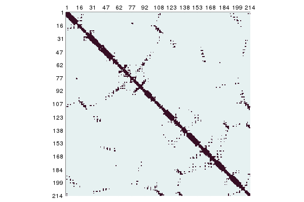
For a quick, text-based representation of a ContactMap use showcontactmap.
DistanceMap works in an analogous way to ContactMap and gives a map of the distances. It can also be plotted:
dists = DistanceMap(collectatoms(struc['A'], cbetaselector))
using Plots
plot(dists)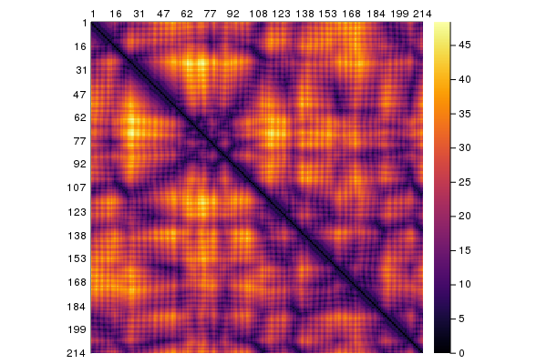
The contacting elements in a molecular structure form a graph, and this can be retrieved using MetaGraph. This extends MetaGraph from MetaGraphs.jl, allowing you to use all the graph analysis tools in LightGraphs.jl. For example:
julia> mg = MetaGraph(collectatoms(struc["A"], cbetaselector), 8.0)
{85, 423} undirected Int64 metagraph with Float64 weights defined by :weight (default weight 1.0)

julia> using LightGraphs, MetaGraphs

julia> nv(mg)
85

julia> ne(mg)
423

julia> get_prop(mg, :contactdist)
8.0

julia> mg[10, :element]
Atom CB with serial 71, coordinates [-3.766, 4.031, 23.526]
See the LightGraphs docs for details on how to calculate properties such as shortest paths, centrality measures, community detection and more. Similar to ContactMap, contacts are found between any element type passed in. So if you wanted the graph of chain contacts in a protein complex you could give a Model as the first argument.
Downloading PDB files
To download a PDB file to a specified directory:
downloadpdb("1EN2", pdb_dir="path/to/pdb/directory")To download multiple PDB files to a specified directory:
downloadpdb(["1EN2", "1ALW", "1AKE"], pdb_dir="path/to/pdb/directory")To download a PDB file in PDB, XML, MMCIF or MMTF format use the file_format argument:
downloadpdb("1ALW", pdb_dir="path/to/pdb/directory", file_format=MMTF)

# To get XML
downloadpdb("1ALW", pdb_dir="path/to/pdb/directory", file_format=PDBXML)
To apply a function to a downloaded file and delete the file afterwards:
downloadpdb(f, "1ALW")Or, using Julia's do syntax:
downloadpdb("1ALW") do fp
    s = read(fp, PDB)
    # Do something
end
Reading PDB files
To parse an existing PDB file into a Structure-Model-Chain-Residue-Atom framework:
julia> struc = read("/path/to/pdb/file.pdb", PDB)
ProteinStructure 1EN2.pdb with 1 models, 1 chains (A), 85 residues, 754 atoms
Read a mmCIF file instead by replacing PDB with MMCIF. Various options can be set through optional keyword arguments when parsing PDB/mmCIF files:
| Keyword Argument | Description |
|---|---|
structure_name::AbstractString | The name given to the returned ProteinStructure; defaults to the file name |
remove_disorder::Bool=false | Whether to remove atoms with alt loc ID not ' ' or 'A'. |
read_std_atoms::Bool=true | Whether to read standard ATOM records. |
read_het_atoms::Bool=true | Whether to read HETATOM records. |
The function readpdb provides an alternative way to read PDB files with a similar interface to downloadpdb. To parse a PDB file by specifying the PDB ID and PDB directory:
struc = readpdb("1EN2", pdb_dir="/path/to/pdb/directory")The same keyword arguments are taken as read above, plus pdb_dir and ba_number.
Use retrievepdb to download and parse a PDB file into a Structure-Model-Chain-Residue-Atom framework in a single line:
julia> struc = retrievepdb("1ALW", pdb_dir="path/to/pdb/directory")
INFO: Downloading PDB: 1ALW
ProteinStructure 1ALW.pdb with 1 models, 2 chains (A,B), 346 residues, 2928 atoms
If you prefer to work with data frames rather than the data structures in BioStructures, the DataFrame constructor from DataFrames.jl has been extended to construct relevant data frames from lists of atoms or residues:
julia> df = DataFrame(collectatoms(struc));

julia> first(df, 3)
3×17 DataFrame. Omitted printing of 5 columns
│ Row │ ishetero │ serial │ atomname │ altlocid │ resname │ chainid │ resnumber │ inscode │ x       │ y       │ z       │ occupancy │
│     │ Bool     │ Int64  │ String   │ Char     │ String  │ String  │ Int64     │ Char    │ Float64 │ Float64 │ Float64 │ Float64   │
├─────┼──────────┼────────┼──────────┼──────────┼─────────┼─────────┼───────────┼─────────┼─────────┼─────────┼─────────┼───────────┤
│ 1   │ false    │ 1      │ N        │ ' '      │ GLU     │ A       │ 94        │ ' '     │ 15.637  │ -47.066 │ 18.179  │ 1.0       │
│ 2   │ false    │ 2      │ CA       │ ' '      │ GLU     │ A       │ 94        │ ' '     │ 14.439  │ -47.978 │ 18.304  │ 1.0       │
│ 3   │ false    │ 3      │ C        │ ' '      │ GLU     │ A       │ 94        │ ' '     │ 14.141  │ -48.183 │ 19.736  │ 1.0       │

julia> df = DataFrame(collectresidues(struc));

julia> first(df, 3)
3×8 DataFrame
│ Row │ ishetero │ resname │ chainid │ resnumber │ inscode │ countatoms │ modelnumber │ isdisorderedres │
│     │ Bool     │ String  │ String  │ Int64     │ Char    │ Int64      │ Int64       │ Bool            │
├─────┼──────────┼─────────┼─────────┼───────────┼─────────┼────────────┼─────────────┼─────────────────┤
│ 1   │ false    │ GLU     │ A       │ 94        │ ' '     │ 9          │ 1           │ false           │
│ 2   │ false    │ GLU     │ A       │ 95        │ ' '     │ 9          │ 1           │ false           │
│ 3   │ false    │ VAL     │ A       │ 96        │ ' '     │ 7          │ 1           │ false           │
Writing PDB files
PDB format files can be written:
writepdb("1EN2_out.pdb", struc)Any element type can be given as input to writepdb. Atom selectors can also be given as additional arguments:
# Only backbone atoms are written out
writepdb("1EN2_out.pdb", struc, backboneselector)
The first argument can also be a stream. To write mmCIF format files, use the writemmcif function with similar arguments. A MMCIFDict can also be written using writemmcif:
writemmcif("1EN2_out.dic", mmcif_dict)Multi-character chain IDs can be written to mmCIF files but will throw an error when written to a PDB file as the PDB file format only has one character allocated to the chain ID.
If you want the PDB record line for an Atom, use pdbline. For example:
julia> pdbline(at)
"HETATM  101  C  A  X B  20      10.500  20.123  -5.123  0.50 50.13           C1+"
If you want to generate a PDB record line from values directly, do so using an AtomRecord:
julia> pdbline(AtomRecord(false, 669, "CA", ' ', "ILE", "A", 90, ' ', [31.743, 33.11, 31.221], 1.00, 25.76, "C", ""))
"ATOM    669  CA  ILE A  90      31.743  33.110  31.221  1.00 25.76           C  "
This can be useful when writing PDB files from your own data structures.
RCSB PDB utility functions
To get the list of all PDB entries:
l = pdbentrylist()To download the entire RCSB PDB database in your preferred file format:
downloadentirepdb(pdb_dir="path/to/pdb/directory", file_format=MMTF)This operation takes a lot of disk space and time to complete (depending on internet connection).
To update your local PDB directory based on the weekly status list of new, modified and obsolete PDB files from the RCSB server:
updatelocalpdb(pdb_dir="path/to/pdb/directory", file_format=MMTF)Obsolete PDB files are stored in the auto-generated obsolete directory inside the specified local PDB directory.
To maintain a local copy of the entire RCSB PDB database, run the downloadentirepdb function once to download all PDB files and set up a CRON job or similar to run updatelocalpdb function once a week to keep the local PDB directory up to date with the RCSB server.
There are a few more functions that may be useful:
| Function | Returns | Return type |
|---|---|---|
pdbstatuslist | List of PDB entries from a specified RCSB weekly status list URL | Array{String,1} |
pdbrecentchanges | Added, modified and obsolete PDB lists from the recent RCSB weekly status files | Tuple{Array{String,1},Array{String,1}, Array{String,1}} |
pdbobsoletelist | List of all obsolete PDB entries | Array{String,1} |
downloadallobsoletepdb | Downloads all obsolete PDB files from the RCSB PDB server | Array{String,1} |
Visualising structures
The Bio3DView.jl package can be used to visualise molecular structures. For example:
using Bio3DView
using Blink
viewpdb("1CRN")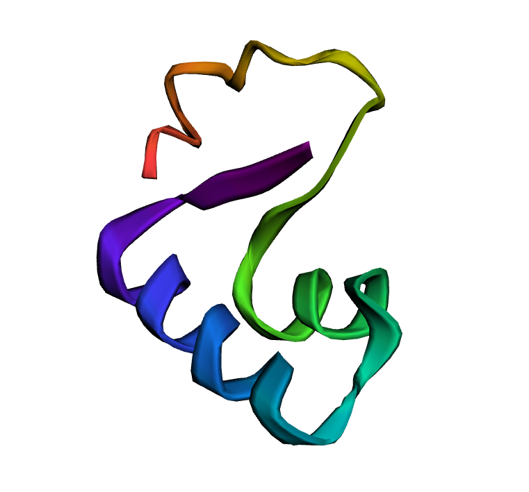
struc = retrievepdb("1AKE")
viewstruc(struc['A'], surface=Surface(Dict("colorscheme"=> "greenCarbon")))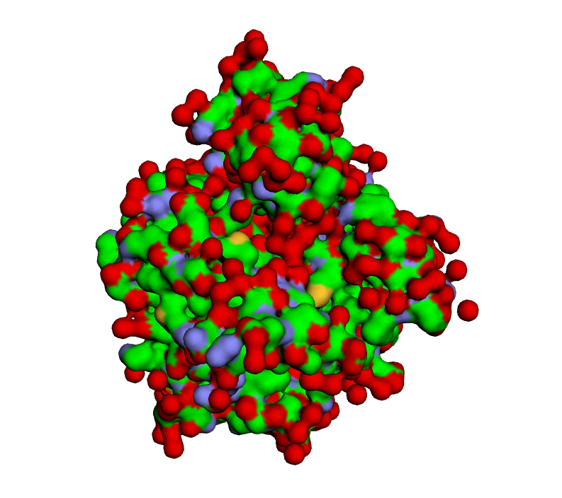
Here they are shown as static images but they are interactive when using Bio3DView.jl. See the Bio3DView.jl tutorial for more information.
Examples
A few further examples of BioStructures usage are given below.
A) Plot the temperature factors of a protein:
using Plots
calphas = collectatoms(struc, calphaselector)
plot(resnumber.(calphas),
     tempfactor.(calphas),
     xlabel="Residue number",
     ylabel="Temperature factor",
     label="")
B) Print the PDB records for all C-alpha atoms within 5 Angstrom of residue 38:
for at in calphas
    if distance(struc['A'][38], at) < 5.0 && resnumber(at) != 38
        println(pdbline(at))
    end
end
C) Find the residues at the interface of a protein-protein interaction:
for res_a in collectresidues(struc["A"], standardselector)
    for res_b in collectresidues(struc["B"], standardselector)
        if distance(res_a, res_b) < 5.0
            println(resnumber(res_a), "A ", resnumber(res_b), "B")
        end
    end
end
D) Show the Ramachandran phi/psi angle plot of a structure:
using Plots
phi_angles, psi_angles = ramachandranangles(struc, standardselector)
scatter(rad2deg.(phi_angles),
     rad2deg.(psi_angles),
     title="Ramachandran plot",
     xlabel="Phi / degrees",
     ylabel="Psi / degrees",
     label="",
     xticks=[-180, -90, 0, 90, 180],
     yticks=[-180, -90, 0, 90, 180],
     xlims=(-180, 180),
     ylims=(-180, 180))
E) Calculate the RMSD and displacements between the heavy (non-hydrogen) atoms of two models in an NMR structure:
downloadpdb("1SSU")
struc_nmr = read("1SSU.pdb", PDB)
rmsd(struc_nmr[5], struc_nmr[10], heavyatomselector)
displacements(struc_nmr[5], struc_nmr[10], heavyatomselector)
F) Calculate the cysteine fraction of every structure in the PDB:
l = pdbentrylist()
for p in l
    downloadpdb(p, file_format=MMCIF) do fp
        s = read(fp, MMCIF)
        nres = countresidues(s, standardselector)
        if nres > 0
            frac = countresidues(s, standardselector, x -> resname(x) == "CYS") / nres
            println(p, "  ", round(frac, digits=2))
        end
    end
end
G) Interoperability is possible with other packages in the Julia ecosystem. For example, use NearestNeighbors.jl to find the 10 nearest residues to each residue:
using NearestNeighbors
struc = retrievepdb("1AKE")
ca = coordarray(struc["A"], cbetaselector)
kdtree = KDTree(ca; leafsize=10)
idxs, dists = knn(kdtree, ca, 10, true)
H) Interoperability with DataFrames.jl gives access to filtering, sorting, summary statistics and other writing options:
using DataFrames
using CSV
using Statistics
struc = retrievepdb("1ALW")
df = DataFrame(collectatoms(struc))
describe(df) # Show summary
mean(df.tempfactor) # Column-wise operations
sort(df, :x) # Sorting
CSV.write("1ALW.csv", df) # CSV file writing