The kinship interface has changed a bit between versions 0.7 and 0.9. This
post has not yet been updated for versions 0.9.0+. To follow along, use versions 0.8.0 or lower.
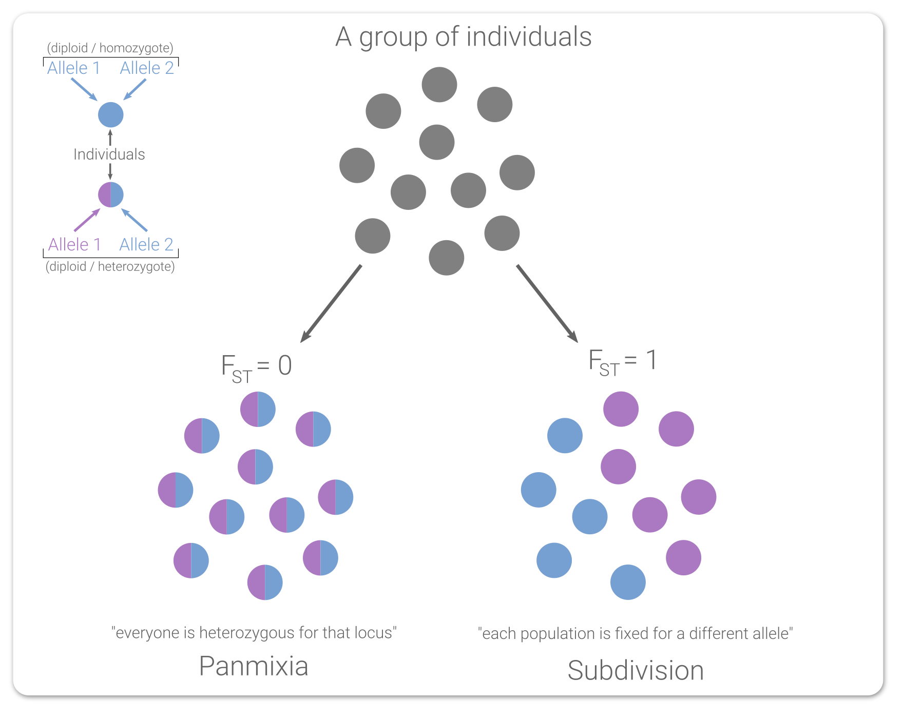
In a population genetics study, you often need to identify if there are kin in your data. This may be necessary because you are trying to remove kin from your data (because of Hardy-Weinberg assumptions), or maybe kinship is a central interest in your study. Either way, the goal of this tutorial is to provide you with a basic tutorial on using PopGen.jl to perform a relatedness analysis, which is sometimes called a kinship analysis. To follow along, you'll need to have Julia, along with the packages PopGen.jl, PopGenSims.jl, and StatsBase.jl installed. We'll be using the nancycats data because it's smaller than gulfsharks, so things should be a lot quicker.
using PopGen, PopGenSims, StatsBase

julia> cats = @nancycats
PopData{Diploid, 9 Microsatellite Loci}
  Samples: 237
  Populations: 17
Like Coancestry and the R packages that wrap it (i.e. relate, related), PopGen.jl provides a whole bunch of relatedness estimators that you can choose from for your data. Unfortunately, there is no right answer and you will need to use your discretion. Some people choose an estimator based on the heterozygosity of the data, others choose one based on more liberal or conservative values, and there are yet more criteria one can consider for choosing an estimator. To keep things simple, we're going to use LynchLi. Why? Because I'm the one writing this tutorial, and I said so 😁.
This seems pretty obvious, but it needs to be said. In order to do the analysis, you need you get the pairwise relatedness values for the individuals of interest in your data. To keep things simple, we're going to do an all-by-all comparison. But, we also want to boostrap the pairs to create confidence intervals ("CI") for each pair, so let's talk about that.
It would behoove us to bootstrap the loci in a pairwise comparison n number of times so we can create a confidence interval for the relatedness estimates for each pair. This inflates the runtime of the analysis substantially, but it's a very useful method in making sense of our estimates. If one was to be conservative (and we generally are), then we would reject an estimate for a pair whose CI includes zero. In PopGen.jl, the estimates and bootstrapping are done all at once to minimize processing time, so the command for that would be
julia> rel_out = kinship(cats, method = LynchLi, iterations = 1000)
By default, the kinship function uses a 95% CI (interval = (0.025, 0.975)), but you can change that with interval = (low,high) where low and high are decimals of your quantiles.
The kinship() function returns a NamedTuple of dataframes whenever you are bootstrapping, where each element shares its name with the method used, so in this case, we can access our results with rel_out.LynchLi.
julia> rel_out.LynchLi
27966×8 DataFrame
   Row │ sample_1  sample_2  n_loci  LynchLi     LynchLi_mean  LynchLi_median  LynchLi_S ⋯
       │ String    String    Int64   Float64?    Float64?      Float64?        Float64?  ⋯
───────┼──────────────────────────────────────────────────────────────────────────────────
     1 │ N215      N216           8   0.743535      0.747288        0.748042     0.75344 ⋯
     2 │ N215      N217           8   0.230605      0.233593        0.240085     0.34187
     3 │ N215      N218           8   0.230605      0.230507        0.221861     0.32161
     4 │ N215      N219           8   0.230605      0.23601         0.23567      0.32782
     5 │ N215      N220           8   0.333191      0.33798         0.350492     0.39898 ⋯
     6 │ N215      N221           8   0.589656      0.594223        0.601308     0.61945
     7 │ N215      N222           8   0.0254328     0.0347216       0.0262021    0.21408
     8 │ N215      N223           8   0.333191      0.329983        0.331411     0.38402
     9 │ N215      N224           8  -0.0258602    -0.021062       -0.0301579    0.21112 ⋯
    10 │ N215      N7             8  -0.282325     -0.27967        -0.288337     0.33611
    11 │ N215      N141           8  -0.0771532    -0.0796867      -0.083113     0.21261
    12 │ N215      N142           8   0.0254328     0.0302549       0.0330718    0.23957
   ⋮   │    ⋮         ⋮        ⋮         ⋮            ⋮              ⋮             ⋮     ⋱
 27955 │ N295      N289           7   0.322731      0.347021        0.34118      0.41168 ⋯
 27956 │ N295      N290           7   0.153414      0.160102        0.164866     0.22862
 27957 │ N296      N297           7  -0.0159038    -0.0182747      -0.0187108    0.16981
 27958 │ N296      N281           7   0.0405353     0.037025        0.0422647    0.15294
 27959 │ N296      N289           7   0.322731      0.328379        0.337317     0.35578 ⋯
 27960 │ N296      N290           7   0.153414      0.152384        0.16194      0.19131
 27961 │ N297      N281           7  -0.0159038    -0.0128349      -0.0303449    0.21030
 27962 │ N297      N289           7   0.37917       0.392517        0.392818     0.45139
 27963 │ N297      N290           7   0.435609      0.437829        0.450044     0.47027 ⋯
 27964 │ N281      N289           8   0.20428       0.21279         0.207425     0.29611
 27965 │ N281      N290           7   0.37917       0.386583        0.390585     0.45471
 27966 │ N289      N290           7   0.209853      0.217811        0.222894     0.28649
                                                          2 columns and 27942 rows omitted
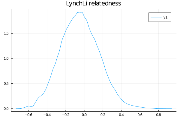
And while it's totally optional, we can plot the distribution of values for some visual data exploration. For that we'll use Plots.jl and StatsPlots.jl.
We could have used any plotting package, but Plots.jl was chosen for simplicity. Other great
options are (and not limited to): Makie.jl, Gadfly.jl, VegaLite.jl, and PlotlyJS.jl.
using Plots, StatsPlots

julia> density(rel_out.LynchLi.LynchLi)
julia> title!("LynchLi relatedness")
The next set of steps seem like a lot more work, so allow me to explain. The estimators all generally give you some value between 0-1 (or 0-0.5, same idea) and you can intuit that certain values mean certain things, like that 0 is "unrelated", 0.25 is "half-sib", and 0.5 is "full-sib". However, those are fixed values, so how do we know how far we can deviate from 0.25 (for example) and still call our pair half-siblings? Instead of hand-waving, we can create confidence intervals from simulated data to act as sibship ranges for our data. If this doesn't make sense yet, it will below. Promise!
Next, we need to further contextualize what out estimates actually mean, and we need to devise a rigorous and defensible method to define the sibling-ship ("sibship") of a pair of samples as unrelated, half-sibs, or full-sibs. To do this, we're going to use PopGenSims.jl to simulate data based on the allele frequencies in our data. What simulatekin does is simulate individuals based on the allele frequencies in your PopData, then simulate offspring of a particular siblingship resulting from the "mating" of those individuals. For example, when you specify "fullsib", it generates two offspring resulting from two parents, n number of times. We want to do this for each of the three kinds of sibships.
julia> kin_sims = simulatekin(cats, fullsib = 500, halfsib = 500, unrelated = 500)
PopData{Diploid, 9 Microsatellite Loci}
  Samples: 3000
  Populations: 3
We can keep all three simulated relationships together, but it will be easier to explain things (for instructional purposes) if we don't, so let's split out each into its own PopData.
julia> fullsib = kin_sims[genodata(kin_sims).population .== "fullsib"] ;
julia> halfsib = kin_sims[genodata(kin_sims).population .== "halfsib"] ;
julia> unrelated = kin_sims[genodata(kin_sims).population .== "unrelated"] ;
Next, we want to get the relatedness estimate for each simulated pair of "known" sibship. We are only interested in the values for the simulated pairs and not samples across pairs. If you aren't sure why that is, think of it this way: we're trying to create a range of values where we can confidently say unknown things are full-sibs (or half-sib, etc.), so we want to know what range of values we get from a bunch of known fullsib pairs, not the unknown relationships of samples between pairs.
It would a nightmare to manually specify only 2 individuals at a time into kinship(). Instead, the function has a shortcut built into it that will recognize the population names generated from simulatekin and only give you relatedness estimates for those pairs. So, we just need to run it once for each of our simulations, this time without bootstrapping because we are only interested in the estimates. Make sure to use the same estimator! The run will be a lot faster this time because it only needs to calculate estimates for 500 pairs each time (our n from above) and without bootstrapping. When not bootstrapping, kinship() returns a dataframe (versus a NamedTuple of dataframes).
- unrelated relatedness
- halfsib relatedness
- fullsib relatedness
julia> un_sims_rel = kinship(unrelated_sims, method = LynchLi)
500×4 DataFrame
 Row │ sample_1            sample_2            n_loci  LynchLi
     │ String              String              Int64   Float64?
─────┼────────────────────────────────────────────────────────────
   1 │ sim001_unrelated_1  sim001_unrelated_2       9  -0.11419
   2 │ sim002_unrelated_1  sim002_unrelated_2       9  -0.337028
   3 │ sim003_unrelated_1  sim003_unrelated_2       9  -0.0696222
  ⋮  │         ⋮                   ⋮             ⋮         ⋮
 498 │ sim498_unrelated_1  sim498_unrelated_2       9   0.019513
 499 │ sim499_unrelated_1  sim499_unrelated_2       9   0.019513
 500 │ sim500_unrelated_1  sim500_unrelated_2       9   0.019513
                                                  494 rows omitted
julia> half_sims_rel = kinship(halfsib_sims, method = LynchLi)
500×4 DataFrame
 Row │ sample_1          sample_2          n_loci  LynchLi
     │ String            String            Int64   Float64?
─────┼────────────────────────────────────────────────────────
   1 │ sim001_halfsib_1  sim001_halfsib_2       9  -0.0182636
   2 │ sim002_halfsib_1  sim002_halfsib_2       9   0.468732
   3 │ sim003_halfsib_1  sim003_halfsib_2       9   0.291643
  ⋮  │        ⋮                 ⋮            ⋮         ⋮
 498 │ sim498_halfsib_1  sim498_halfsib_2       9   0.42446
 499 │ sim499_halfsib_1  sim499_halfsib_2       9   0.513004
 500 │ sim500_halfsib_1  sim500_halfsib_2       9   0.0702811
                                              494 rows omitted
julia> full_sims_rel = kinship(fullsib_sims, method = LynchLi)
500×4 DataFrame
 Row │ sample_1          sample_2          n_loci  LynchLi
     │ String            String            Int64   Float64?
─────┼──────────────────────────────────────────────────────
   1 │ sim001_fullsib_1  sim001_fullsib_2       9  0.732808
   2 │ sim002_fullsib_1  sim002_fullsib_2       9  0.599213
   3 │ sim003_fullsib_1  sim003_fullsib_2       9  0.376553
  ⋮  │        ⋮                 ⋮            ⋮        ⋮
 498 │ sim498_fullsib_1  sim498_fullsib_2       9  0.376553
 499 │ sim499_fullsib_1  sim499_fullsib_2       9  0.510149
 500 │ sim500_fullsib_1  sim500_fullsib_2       9  0.109361
                                            494 rows omitted
And if we wanted to plot what that looks like (optional):
using Plots, StatsPlots

julia> density(rel_out.LynchLi.LynchLi, label = "real data", color = :grey, fill = (0, :grey))
julia> density!(un_sims_rel.LynchLi, label = "unrelated")
julia> density!(half_sims_rel.LynchLi, label = "halfsib", color = :blue)
julia> density!(full_sims_rel.LynchLi, label = "fullsib", color = :black)
julia> title!("relatedness estimates on simulated and real data")
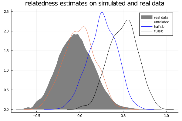
Hopefully by now you are starting to contextualize why we're doing all of this. The distributions generated from our simulated data are giving us a better indication of what "unrelated", "halfsib", and "fullsib" estimates look like in our data.
What we just did is create null distributions for each sibship relationship, so now all that's left is to get a confidence interval from each. Keep in mind that your values will be a bit different due to the randomization involved with many of these steps.
julia> unrelated_ci = quantile(un_sims_rel.LynchLi, (0.025, 0.975))
(-0.3380513384854698, 0.33097433075726507)

julia> halfsibs_ci = quantile(half_sims_rel.LynchLi, (0.025, 0.975))
(-0.06652262584414452, 0.5556155725649398)

julia> fullsibs_ci = quantile(full_sims_rel.LynchLi, (0.025, 0.975))
(0.1989727186688347, 0.8219939374819633)
So, given our data and the simulations we made, we can now make a reasonable assumption regarding the ranges for each sibship relationship:
| Relationship | Lower Bound | Upper Bound |
|---|
| unrelated | -0.338 | 0.331 |
| half sibling | -0.066 | 0.555 |
| full sibling | 0.199 | 0.82 |
Now that we have our relatedness estimates and the acceptable sibship ranges given our data, we can see where our data falls.
Now, we can say that a particular sample pair is unrelated/halfsib/fullsib if:
- that pair's confidence interval does not include zero and
- that pair's estimate falls within any of the three calculate ranges
Unfortunately, the ranges overlap quite a bit, which makes interpretation difficult, so it may be suitable to use a different estimator.
There is more that can be done for relatedness, like network analysis. However, this tutorial covers what we consider a reasonable way to assess kinship in population genetic studies. If removing kin is your ultimate goal, consider the effects doing that may have on the analyses you are looking to do. Additionally, consider which individual of a pair you would remove and why. If you were curious as to how many identical loci a pair of samples may share, you can check that using pairwiseidentical(). Good luck!