Hardy-Weinberg Equilibrium

Testing for Hardy-Weinberg Equilibrium (often abbreviated HWE) is a fairly common practice in population genetics. In a two-allele system, the HWE equation is defined as: $p^2 + 2pq + q^2 = 1$ , where $p$ is the frequency of the first allele and $q$ is the frequency of the second allele. The formula describes the frequency of all possible genotypes where

HWE variable	Genotype	State
$p^2$	"pp"	homozygous
$q^2$	"qq"	homozygous
$2pq$	"pq"	heterozygous

Testing for deviation from HWE is usually done with a Chi-Squared ($\chi^2$) test, where one compares the observed genotype frequencies to the expected genotype frequencies given the observed allele frequencies at a locus. Specifically, the equation is

$$\sum{\frac{(observed - expected)^2}{expected}}$$

where $observed$ is the observed genotype frequency and $expected$ is the expected genotype frequency for a locus. To generate our test statistic, we calculate the degrees of freedom:

$$degrees\ of\ freedom = n_{expected\ genotypes} - n_{observed\ alleles}$$

and use this as the parameter for our $\chi^2$ distribution, followed by a cumulative density function using this $\chi^2$ distribution and our $\chi^2$ value calculated above.

Chi-Squared Test

hwetest(data::PopData, by::String = "locus", correction::String = "none")

Calculate chi-squared test of HWE for each locus and returns observed and expected heterozygosity with chi-squared, degrees of freedom and p-values for each locus. Use by = "population" to perform this separately for each population (default: "locus"). Use correction = to specify a P-value correction method for multiple testing (recommended). For convenience, the correction method is appended to the name of the column, so you will always know how those P-values were adjusted.

Arguments

• data : the input PopData

Keyword arguments

• by : "locus" (default) or "population"
• correction : a string specifying a P-value adjustment type (default: "none")

correction methods

• "bonferroni" : Bonferroni adjustment
• "holm" : Holm adjustment
• "hochberg" : Hochberg adjustment
• "bh" : Benjamini-Hochberg adjustment
• "by" : Benjamini-Yekutieli adjustment
• "bl" : Benjamini-Liu adjustment
• "hommel" : Hommel adjustment
• "sidak" : Šidák adjustment
• "forwardstop" or "fs" : Forward-Stop adjustment
• "bc" : Barber-Candès adjustment

🤔 For more information on multiple testing adjustments, see MultipleTesting.jl

Examples

HWE Chi-Sq

julia> hwetest(@gulfsharks)
2209×4 DataFrame
  Row │ locus         chisq      df     P           
      │ String        Float64    Int64  Float64     
──────┼─────────────────────────────────────────────
    1 │ contig_35208   94.5678       6  0.0
    2 │ contig_23109   50.789        2  9.36085e-12
    3 │ contig_4493    40.7903       2  1.38832e-9
    4 │ contig_10742   14.7325       2  0.000632247
    5 │ contig_14898   58.1948       2  2.30704e-13
    6 │ contig_8483     4.05732      2  0.131511
    7 │ contig_8065    18.0799       2  0.000118574
    8 │ contig_14708   13.6264       2  0.00109919
  ⋮   │      ⋮            ⋮        ⋮         ⋮
 2203 │ contig_18959  106.658        2  0.0
 2204 │ contig_43517   23.8965       2  6.47041e-6
 2205 │ contig_27356   14.4493       2  0.000728417
 2206 │ contig_475     76.6038       2  0.0
 2207 │ contig_19384   13.7915       2  0.00101209
 2208 │ contig_22368   20.3787       2  3.75686e-5
 2209 │ contig_2784     6.13433      2  0.0465531
                                   2194 rows omitted

HWE with P adjustment

julia> hwetest(@gulfsharks, correction = "bh")
2209×5 DataFrame
  Row │ locus         chisq      df     P            P_bh        
      │ String        Float64    Int64  Float64      Float64     
──────┼──────────────────────────────────────────────────────────
    1 │ contig_35208   94.5678       6  0.0          0.0
    2 │ contig_23109   50.789        2  9.36085e-12  2.85215e-11
    3 │ contig_4493    40.7903       2  1.38832e-9   3.62505e-9
    4 │ contig_10742   14.7325       2  0.000632247  0.00102164
    5 │ contig_14898   58.1948       2  2.30704e-13  7.91345e-13
    6 │ contig_8483     4.05732      2  0.131511     0.143532
    7 │ contig_8065    18.0799       2  0.000118574  0.000204314
    8 │ contig_14708   13.6264       2  0.00109919   0.00170656
  ⋮   │      ⋮            ⋮        ⋮         ⋮            ⋮
 2203 │ contig_18959  106.658        2  0.0          0.0
 2204 │ contig_43517   23.8965       2  6.47041e-6   1.27163e-5
 2205 │ contig_27356   14.4493       2  0.000728417  0.00116769
 2206 │ contig_475     76.6038       2  0.0          0.0
 2207 │ contig_19384   13.7915       2  0.00101209   0.00160958
 2208 │ contig_22368   20.3787       2  3.75686e-5   6.82475e-5
 2209 │ contig_2784     6.13433      2  0.0465531    0.0561375
                                                2194 rows omitted

HWE by population

julia> hwetest(@gulfsharks, by = "population")
15463×5 DataFrame
   Row │ locus         population     chisq     df     P                 
       │ String        String         Float64   Int64  Float64?          
───────┼─────────────────────────────────────────────────────────────────
     1 │ contig_35208  CapeCanaveral   6.47676      2        0.0392275
     2 │ contig_35208  Georgia        15.7481       2        0.000380481
     3 │ contig_35208  SouthCarolina  14.2857       2        0.00079049
     4 │ contig_35208  FloridaKeys    27.1399       6        0.000136324
     5 │ contig_35208  MideastGulf    16.6453       2        0.000242956
     6 │ contig_35208  NortheastGulf  10.7263       6        0.0972136
     7 │ contig_35208  SoutheastGulf   8.62222      2        0.0134186
     8 │ contig_23109  CapeCanaveral   6.19376      2        0.0451901
   ⋮   │      ⋮              ⋮           ⋮        ⋮            ⋮
 15457 │ contig_2784   CapeCanaveral   0.0          0  missing           
 15458 │ contig_2784   Georgia         0.0          0  missing           
 15459 │ contig_2784   SouthCarolina   0.0          0  missing           
 15460 │ contig_2784   FloridaKeys     3.11065      2        0.211121
 15461 │ contig_2784   MideastGulf     2.11686      2        0.346999
 15462 │ contig_2784   NortheastGulf   0.0          0  missing           
 15463 │ contig_2784   SoutheastGulf   1.04091      2        0.594251
                                                       15448 rows omitted

When doing this test by population, you may notice some loci have missing P-values for certain populations, indicating that this locus is missing for that population.

Interpreting the results

Since the results are in table form, you can easily process the table using DataFramesMeta.jl or Query.jl to find loci above or below the alpha threshold you want. As an example, let's perform an HWE-test on the nancycats data without any P-value adjustments:

julia> ncats_hwe = hwetest(@nancycats , by = "population") ;

Now, we can now filter this table and leave only what we're interested in:

julia> ncats_hwe[(ncats_hwe.P .!== missing) .& (ncats_hwe.P .<= 0.05), :]

With this command, we filter the table for:

1. the P-values are not missing
2. the P-values are less than or equal to 0.05.

Note: You can use DataFramesMeta.jl, Query.jl, SplitApplyCombine.jl and others for more declarative dataframe manipulation.

This results in a table that now only includes non-missing P-values of 0.05 or lower:

71×5 DataFrame
 Row │ locus   population  chisq     df     P           
     │ String  String      Float64   Int64  Float64?    
─────┼──────────────────────────────────────────────────
   1 │ fca8    2            74.3426     30  1.24317e-5
   2 │ fca8    3            85.2        42  9.15914e-5
   3 │ fca8    6            70.4136     42  0.00390639
   4 │ fca8    7            63.3673     30  0.00035342
   5 │ fca8    10           26.4489     12  0.00926812
   6 │ fca8    11           60.801      42  0.0302593
   7 │ fca8    16           26.15       12  0.0102213
   8 │ fca8    17           57.2        30  0.00198256
  ⋮  │   ⋮         ⋮          ⋮        ⋮         ⋮
  65 │ fca96   16           37.0033     20  0.0116913
  66 │ fca37   1            12.6562      6  0.0488314
  67 │ fca37   3            24.1481     12  0.0194174
  68 │ fca37   5            61.1317     12  1.40268e-8
  69 │ fca37   7            13.0062      6  0.042938
  70 │ fca37   11           61.8056     42  0.024858
  71 │ fca37   12           61.618      42  0.0257958
                                         56 rows omitted

Visualizing the results

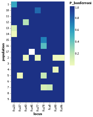
While not strictly necessary, it might sometimes make sense to generate of heatmap of the results for easier visualization. This is feasible for the nancycats data, but when loci are in the hundreds or thousands, this method quickly becomes counterproductive. In any case, here is a simple example of the HWE results for nancycats plotted as a heatmap using VegaLite.jl (other packages like Makie.jl, Plots.jl, Gadfly.jl etc. would work great too!):

using VegaLite

julia> ncats_hwe = hwetest(@nancycats , by = "population", correction = "bonferroni");

julia> ncats_hwe |> @vlplot(:rect, :locus, :population, color=:P_bonferroni)

---

Acknowledgements

While most of the arithmetic for the Hardy-Weinberg test is written by us, we rely on the Chi-Squared distribution and probability density function provided by Distributions.jl.