t-SNE

t-distributed stochastic neighbor embedding (a.k.a. t-SNE) is a dimensionality reduction technique for visualizing high-dimensional data. It does this by giving each datapoint a location in a two or three-dimensional map by minimizing the Kullback–Leibler divergence between the high and low dimensionality probability distributions with respect to the locations of the points in the map. It models each high-dimensional object by a two- or three-dimensional point so similar objects are appear nearer and dissimilar objects appear further apart. Read more about it here.

PopGen.jl v0.10x removed TSNE.jl as a dependency and instead this page is inteded to walk you through how to use PopGen.jl and TSne.jl together. You will need to install TSne.jl with

julia> ]add TSne
# or #
julia> using Pkg; Pkg.add("TSne")

warning

Visual clusters can be seriously influenced by the parameters. For example, parameters can be chosen in such a way to identify clusters in data that has none. So, a good understanding of the parameters for t-SNE is necessary. Although a useful tool, t-SNE is not commonly used in population genetic analysis. It is included here due to its utility in adjacent disciplines.

Step 1: Create the allele frequency matrix

You will need to input an allele frequency matrix into the tsne function. fortunately, PopGenCore.jl has the a matrix method to do that. Missing values in the matrix will be replaced with the global mean frequency of that allele.

julia> using TSne
julia> cats = @nancycats;
julia> mtx = matrix(cats, missings = "mean")
237×108 Matrix{Float64}:
00230415  0.00230415  …  0.0  0.0  0.0
00230415  0.00230415     0.0  0.0  0.0
0         0.0            0.0  0.0  0.0
0         0.0            0.0  0.0  0.0
0         0.0            0.0  0.0  0.0
0         0.0         …  0.0  0.0  0.0
0         0.0            0.0  0.0  0.0
 ⋮                       ⋱  ⋮         
0         0.0            0.0  0.0  0.0
0         0.0            0.5  0.0  0.0
0         0.0            0.0  0.0  0.0
0         0.0            0.0  0.0  0.0
0         0.0         …  0.0  0.0  0.0
0         0.0            0.0  0.0  0.0

Step 2: Perform t-SNE on the frequency matrix

The method signature for tsne is:

tsne(mtx, ndim, reduce_dims, max_iter, perplexity; kwargs...)

Arguments

mtx: the allele frequency matrix
ndim: dimension of the embedded space (default: 2)
reduce_dims the number of the first dimensions of X PCA to use for t-SNE, if 0, all available dimension are used (default: 0)
max_iter: how many iterations of t-SNE to do (default: 1000)
perplexity: the perplexity is related to the number of nearest neighbors that is used in other manifold learning algorithms. Larger datasets usually require a larger perplexity. Consider selecting a value between 5 and 50. Different values can result in significantly different results (default: 30)

Keyword Arguments (optional)

distance: if true, specifies that X is a distance matrix, if of type Function or Distances.SemiMetric, specifies the function to use for calculating the distances between the rows (or elements, if X is a vector) of X
pca_init: whether to use the first ndims of X PCA as the initial t-SNE layout, if false (the default), the method is initialized with the random layout
verbose if true, output informational and diagnostic messages
progress: if true, display progress meter during t-SNE optimization
min_gain, eta, initial_momentum, final_momentum, momentum_switch_iter, stop_cheat_iter, cheat_scale: low-level parameters of t-SNE optimization
extended_output: if true, returns a tuple of embedded coordinates matrix, point perplexities and final Kullback-Leibler divergence

Once you have the allele frequency matrix, you just plug it into tsne from TSne.jl as the first positional argument.

julia> results_tsne = tsne(mtx, 5, 0, 100)
237×5 Matrix{Float64}:
  2.33077   -0.313104   …   0.261691
 -1.41855   -1.16244        3.90946
  0.181728  -0.15139       -0.0399188
 -1.24196    0.676003       0.567271
 -1.94341   -0.221126       2.64668
 -1.87612   -0.280161   …  -0.272155
 -0.283864   0.322579      -0.181031
  ⋮                     ⋱  
 11.3574     7.64794       -0.495769
  8.05785    1.7843         5.63656
 -0.23807    0.729471      -0.0126313
 -0.264675  -0.0643155     -1.40175
  5.07462   -0.467093   …   1.40149
 -4.76319    7.16874        9.06195

Step 3: Nicer formatting for results

The results can look like a nice legible dataframe with this code snippet. You may need to import DataFrames, since PopGen.jl doesn't reexport the DataFrame function.

julia> df_tsne = DataFrame(results_tsne, String["dim"*"$i" for i in 1:size(results_tsne, 2)]); 
julia> insertcols!(df_tsne, 1, :name => samplenames(cats), :population => cats.sampleinfo.population)
237×7 DataFrame
 Row │ name     population  dim1        dim2        dim3        ⋯
     │ String7  String      Float64     Float64     Float64     ⋯
─────┼───────────────────────────────────────────────────────────
   1 │ N215     1            2.33077    -0.313104    1.15179    ⋯
   2 │ N216     1           -1.41855    -1.16244     4.58651
   3 │ N217     1            0.181728   -0.15139     0.813046
   4 │ N218     1           -1.24196     0.676003   -0.805543
   5 │ N219     1           -1.94341    -0.221126    0.443529   ⋯
   6 │ N220     1           -1.87612    -0.280161   -1.11817
   7 │ N221     1           -0.283864    0.322579   -0.425085
   8 │ N222     1            5.43832    11.368       0.727039
  ⋮  │    ⋮         ⋮           ⋮           ⋮           ⋮       ⋱
 231 │ N294     17           5.34851    -2.43159     0.685094   ⋯
 232 │ N295     17          11.3574      7.64794    13.1644
 233 │ N296     17           8.05785     1.7843     -8.18657
 234 │ N297     17          -0.23807     0.729471    0.548891
 235 │ N281     17          -0.264675   -0.0643155   0.0122561  ⋯
 236 │ N289     17           5.07462    -0.467093    0.0678861
 237 │ N290     17          -4.76319     7.16874    -7.3478
                                   2 columns and 222 rows omitted

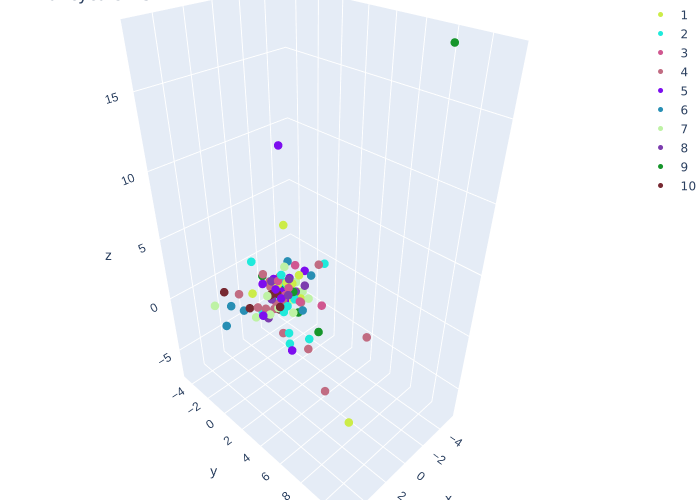
Step 4: Make fancy 3D plot

People tend to like plotting PCA and t-SNE as 3-dimensional scatterplots because you can see, well, 3 dimensions at once. Below is a code snippet that uses PlotlyJS.jl to make an interactive 3-dimensional scatterplot of the t-SNE results. It's not the most intuitive plotting library in Julia (can use Plots.jl with a plotly backend, or GLMakie), but both of those have large dependencies that would be a big ask for a simple tutorial.

using PlotlyJS

function tsne_plot(data::DataFrame)
    # load data and restrict to just 10 populations for simplicity
    pops = unique(data.population)[1:10]
    colors = ["#ccec48","#1feadb","#d05790","#c16c82","#7d0eef", "#288fb4","#bef2a5", "#7c3dae", "#16952b", "#772932"]
    plotdat = GenericTrace[]

    for (i, nm) in enumerate(pops)
        df = data[data.population .== nm, :]
        x=df.dim1
        y=df.dim2
        z=df.dim3
        trace = scatter3d(;
          name = nm,
          mode = "markers",
          marker_size = 5,
          marker_color = colors[i],
          marker_line_width = 0,
          x = x,
          y = y,
          z = z
        )
        push!(plotdat, trace)
    end
    layout = Layout(
      margin=attr(l=0, r=0, t=0, b=0),
      title = "Nancycats t-SNE",
      xaxis=attr(title="Dimension 1"),
      yaxis=attr(title="Dimension 2"),
      zaxis=attr(title="Dimension 3")
      )
    plot(plotdat, layout)
end

tsne_plot(df_tsne)

tnse plot

Step 1: Create the allele frequency matrix​

Step 2: Perform t-SNE on the frequency matrix​

Arguments​

Keyword Arguments (optional)​

Step 3: Nicer formatting for results​

Step 4: Make fancy 3D plot​